Edit alarm limit (job)
Static alarm limits
After creating a job one should set suitable thresholds to represent its current status depending on the measured values. The alarm limits section can be accessed directly by selecting Edit -> Alarm limits from a job’s dropdown list or by clicking “OK, Edit Alarm limits” in the toolbar after the job’s details have been configured:

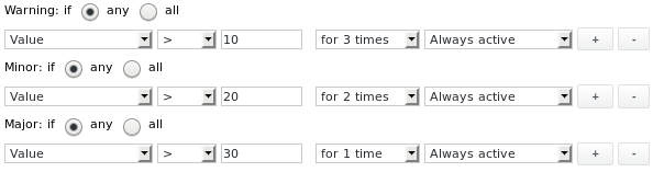
At job creation default alarm limits are set depending on job type (see section Available plugins), for example a new Icmp job has the following alarm limits configured by default:
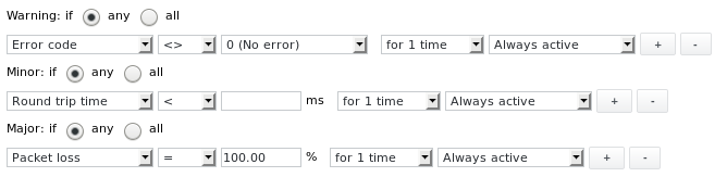
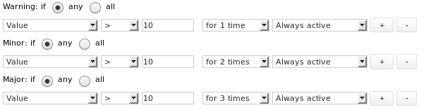
Separate alarm limits can be set for each of the 3 states Warning, Minor or Major.
To add new thresholds click the + button. If more then one alarm limit is configured for a specific state, set their correlation by choosing either of the any or all radio buttons. When all is selected, all thresholds must be fulfilled to change the state of the job. Click the - button to remove a threshold.
Adding an additional Minor threshold to the example above:
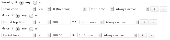
In this example a Minor alarm is only triggered if the round trip time of the icmp check has been above 200 ms for the last 3 job executions.
Job alarm state examples
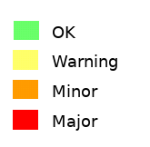
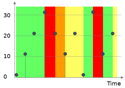
The following example state history plots show how a job's state change for different configurations of alarm limits and their counters. The following state colours are used:
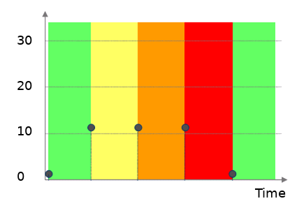
Same limits, increasing counters
Configure the for x times parameter to define how often a value must be over the limit, as a job turns to the particular not OK state. With the first value below the limit, the job turns back to OK.
|
|
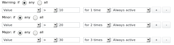
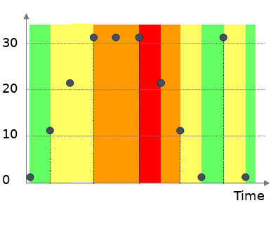
Increasing limits, increasing counters
For increasing values, the state changes when the value is n-times over the particular limit. The same happens to the decreasing values.
|
|
Increasing limits, decreasing counters
For increasing and decreasing values, the state changes when the value is n-times over the particular limit. If no condition is valid the job turns back to OK.
|
|
Value-dependent maintenance on parsefile jobs
If an input file contains information about the maintenance state of a certain device or object, this can be parsed by a parsefile job on the device object and depending on the findings of the parse sequence the parsefile job can be put into Maintenance state or not. Parsefile jobs offer the additional Maintenance threshold to allow setting the job under Maintenance:
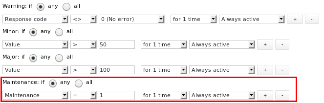
A job that is under Maintenance propagates its Maintenance state upward to its device. The device object itself then propagates the Maintenance state downwards to all its jobs.
Time-dependent alarm limits
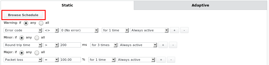
By default the configured thresholds are Always active which means that no specific schedule is assigned. Using a schedule, time-dependent thresholds can be configured. This is useful in case one would like to establish different sensitivity levels for alarming within or outside operating hours or during the usual maintenance windows. By configuring a schedule for a job's alarm limits, the job's execution is still governed by its execution interval, only its state and thus its alarming functionality are time-dependent.
To set time-dependent alarm limits, a schedule may be assigned to each alarm limit entry. First, click the Browse Schedule button to browse for the schedule object. All existing schedule objects can be found under /root/Configurations/Schedule. Select one or several schedules using the checkboxes, then click Next:
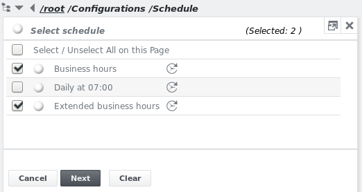
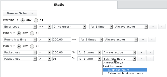
Now the selected schedules are available in the dropdown list on each of the alarm limits:
If a referenced schedule object is deleted, the reference for the threshold changes to Always active.
If the definition of a schedule is changed, the alarm limit in a history plot is displayed using the new definition of the schedule. This applies although the corresponding states have been calculated using the definition valid before the change was performed. History plots do not reflect the history of configuration objects.
Variable alarm limits with external timestamp source
Static alarm limits work well for systems that have no human interaction. In situations, where a timestamp in a file is only updated if a human takes action the timestamp will not be adjusted on public holidays or weekends. A file that is updated regularly during business hours may not be older than 24 hours, but might easily be older than 60 hours on a weekend - not to mention what happens if a public holiday is adjacent to a weekend. To handle such situations a variable timestamp check can be used.
Some plugin types (e.g. the Execute or Parsefile plugins) support reading the timestamp from an external source.
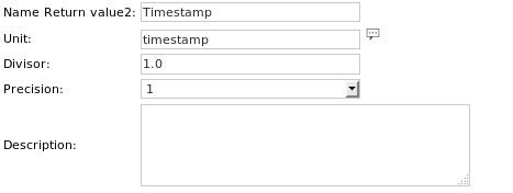
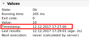
The timestamp can be provided as an absolute number of seconds since 1.1.970 (UNIX epoch time) or as variable age in seconds. If the former method is used the Unit name can be defined with the magic word timestamp and the rather unreadable number will be automatically transformed to a human readable string:
The corresponding configuration for a variable alarm limit looks like this:

Instead of a static limit of e.g. 1h a special string is entered like =1h+132. The "=" sign marks a variable alarm limit. The following string expresses the desired age and the +132 states the ID of the schedule to be added. See chapter Schedule and exception schedule for information on how to create a schedule.
Adaptive alarm limits
Alarm limits can also be set based on the standard deviation (σ) or a percental deviation. The values measured by a job can be considered for alarming. This can be useful in cases where a job's value follows a more or less regular weekly trend. For example the disk and CPU usage on a device that runs local backup jobs each sunday rise during the backups and settle to normal levels after the backups have finished. One would like to recognize those cases where the disk or CPU usage values deviate from this normal behaviour, e.g. when the disk usage rises significantly when no backup windows are active. Another example for using adaptive alarm limits might be an online transaction system which usually has a high load during daytime and a very low load during the night or over the weekend. Adaptive alarm limits can help detect anomalies in this behavior.
In cases where a more or less linear trend is discernible in a value history, e.g. when disk usage rises continuously on a file server's disk volume, one might like to be notified a certain number of days or weeks in advance, before the disk usage level reaches a certain value. Just so one can go and buy additionaly disks to grow the storage volume.
The σ and % operators, as well as the Anticipated items, can be used for the above purposes:
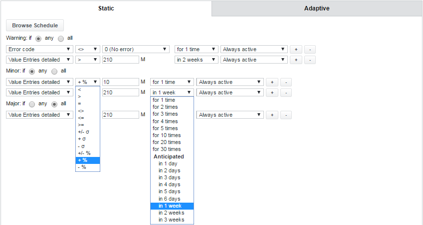
Don't combine the σ or % alarm limit operators with the Anticipated function (on the same alarm limit line). Use them on data that has a low correlation coefficient but shows regular weekly trends.
These adaptive alarm limits can also be combined with static alarm limits.
Please note that SKOOR Engine will need some time to calculate prediction data. During this time, it will show the following message in the header section of the UI as long as the Adaptive tab is selected:

Alarm limits with Anticipated values
Switch to the Adaptive tab to see the history values, the calculated mean time series and the corresponding alarm limits projected into the future. The following example shows the Adaptive tab with the last 14 days of a value history (blue line) with an almost perfectly linear trend:
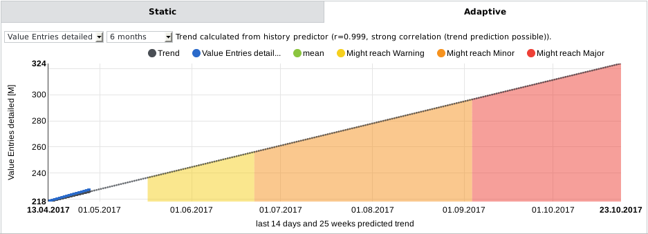
The correlation coefficient calculated from the data is shown on top of the graph. The trend of the actually measured data is projected into the future for the next 25 weeks. This corresponds to the gray Trend line. The time range into the future can be chosen from the second dropdown list.
The following alarm limits have been set for the above example:
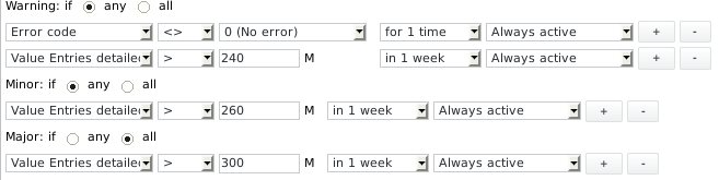
One can see that 1 week before the value 240 will be reached (as expected from the current trend), the job will assume the Warning state. The same goes for the Minor and Major states.
Standard deviation (σ) and percental deviation
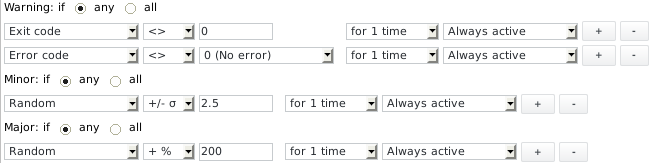
For measured values that don't follow such a clear linear trend, i.e. that show a lower correlation coefficient, the σ- or %-alarm limits can be set:
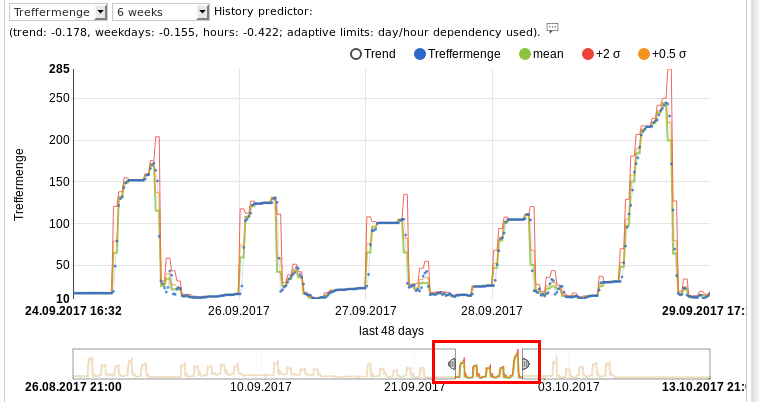
This example shows a weekly pattern with significantly lower values on weekends. In such cases a prediction is not possible because the measured values are spread over a wide range, but the Adaptive tab visualizes this scattering and combines it with the alarm limits currently configured:
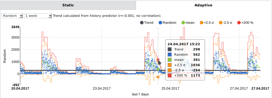
The graph in the Adaptive tab can appear in two different ways depending on the calculated correlation. If the correlation coefficient r is higher than 0.3, the hour/day-dependent calculation is used and a trend focused graph will be shown as in section Alarm limits with Anticipated values. Separate correlation coefficients are then calculated for hourly and daily data. If it is lower, the graph shows a view of the calculated alarm limits based on historic data only (with no prediction into the future), as seen above.
Should the Random value be abnormally high on the next weekend, e.g. as high as on normal weekdays, then this would trigger either the +2.5 σ and/or the +200% alarm limit and the job's state would turn Minor or even Major.
The job generates an alarm as soon as measured values are outside the predicted values calculated from historic data. Practically, this means that the last 5 weeks of data are considered for the calculation of the statistics with reduced weighting towards weeks longer ago.
The alarm limits can also be viewed from the job's value history. See section Show value history for details.
Individual curves in the graph above can be hidden by clicking the round button with the corresponding colour. E.g. clicking the black Trend button hides the trend line.
Selecting the time range
Below the graph in the Adaptive tab there's a timeline of the whole time range that was configured in the dropdownlist on top of the graph (1 week in this example). Here one can specify the time range to show in the main graph by selecting a time range with the mouse:
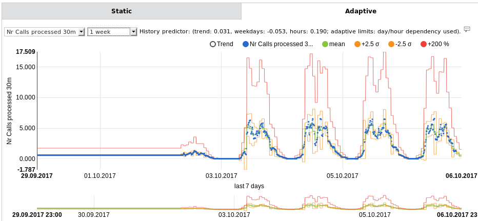
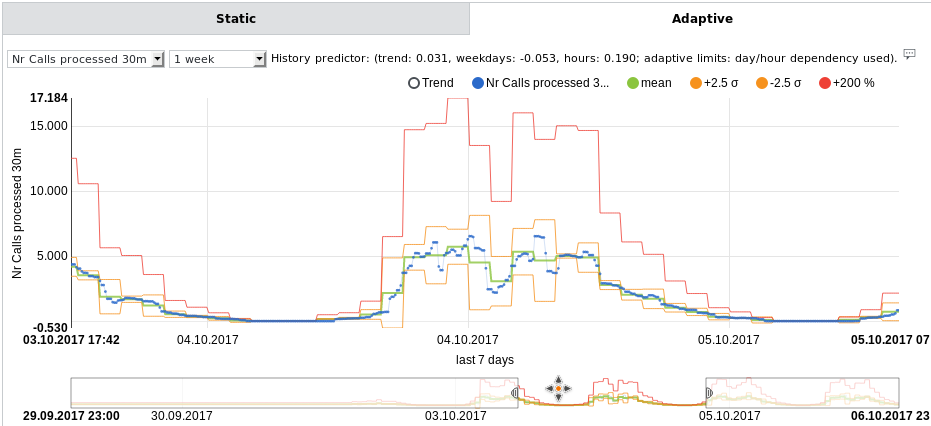
The time range below the cursor is shown as a zommed section above. It can be adjusted on each end or moved to the left or right.
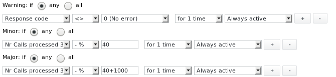
Offset for percental alarm limits
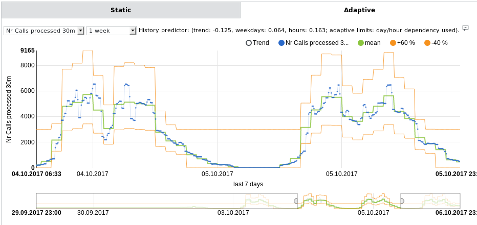
Sometimes the percental alarm limit is triggered even if the current values show a very similar trend as in previous weeks. This is often the case during times when the steepness of the value curve is very high. In such cases, the percental alarm limits can be enhanced with a numerical static offset. The following example shows a value curve (blue) where alarm limits were configured for Minor and Major state, both with a threshold of -40%, but the Major alarm limit was configured with an additional offset of 1000. The offset is configured by appending it to the percental value with a + character.
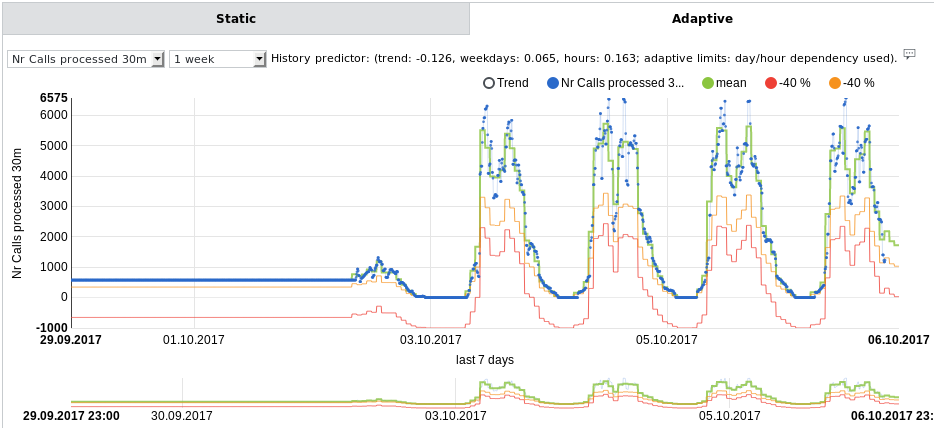
The offset pushes the red Major threshold curve 1000 units (in this case: calls) downwards, so the Major threshold is not reached easily during the steep onset of the rising value.
Limit for percental alarm limits
Sometimes one would like to use percental thresholds, but wants to make sure that there's still a hard maximum limit at a certain value. The following example shows a value curve (blue) where alarm limits were configured for Minor state. One positive and one negative percental limit with each a hard limit of 1000 and 3000 units respectively. Such limits are configured by appending the static limit to the percental value with a > character.
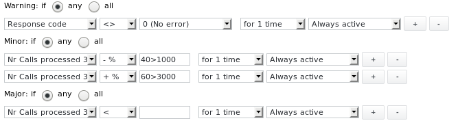
This means that the negative limit of 40% is set to 0 if the calculated limit would be less than 1000 and the positive limit of 60% is set to a minimum of 3000 if the calculated limit would be less than 3000, respectively.
Schedule for adaptive alarm limits
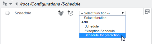
Since adaptive alarm limits try to adapt day-dependent loads, it may be necessary to account for known anomalies like holidays. If a system has high load every Friday, but on Good Friday very low load or even no load at all is assumed, there needs to be a way to teach the system that Good Friday is not a normal Friday but will behave like a Sunday. To achieve this, a special kind of schedule can be configured. See Section Schedule for prediction for more information.
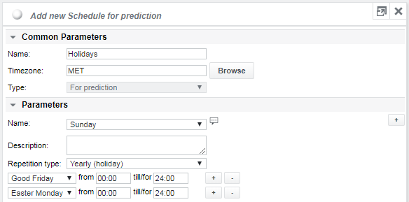
Create a Schedule for prediction:
In the following example, on Good Friday and Easter Monday, the adaptive alarm limits calculated from the last Sunday loads will be applied:
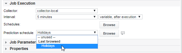
Now link this schedule to jobs with adaptive alarm limits by browsing and selecting the schedule using the Prediction schedule dropdown:
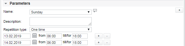
One may also configure one time changes to the alarm limits, by selecting One time instead of Yearly (holiday) from the Repetition type dropdown list:
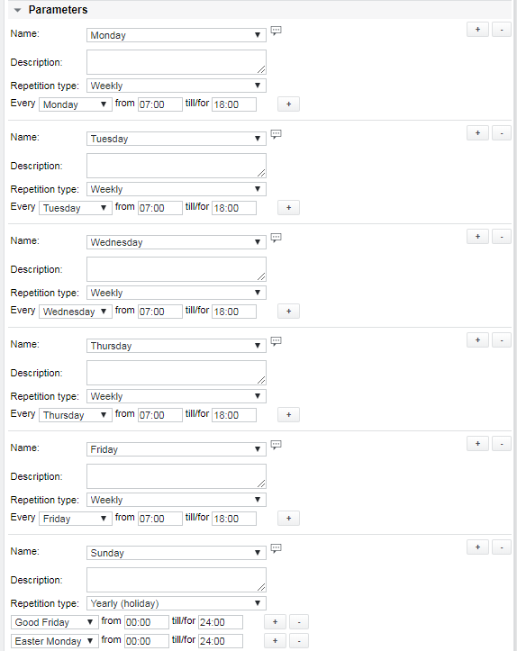
These schedule parameters can also be combined with ordinary active schedules inside the same schedule object. The following figure shows an example of an active schedule which defines business hours for alarming and also specifies that Good Friday and Easter Monday are to be trated as Sundays for adaptive alarm limit calculations:
Fixing job values with wrong or missing measurements
Sometimes a job's values have been tainted by misconfiguration on the job's parameters (e.g. a wrong value was selected leading to extremely high or low values) or due to the job not having been active and measuring when it should have. In the following example a job was not doing any correct measurements anymore since somewhere around October 6th. The incorrect values negatively impact the statistics calculation:
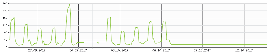
In such a case, data can be invalidated. In the example above, the time range between October 6th and October 14th will be invalidatedd and not considered for adaptive alarm limit calculation anymore.
The reqired time range may be specified in the time selector below the graph:
Two buttons will be visible below the selector, one to invalidate and one to validate data in the selected time range:

After Invalidate or Validate was clicked and confirmed, the time selector shows the respective time ranges with red marks: 
Also, the Recalculate prediction data button becomes visible. This button must be clicked to calculate the prediction data with the changed values:

Targets
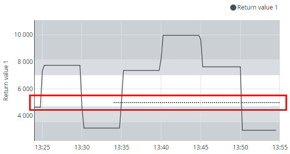
A special type of alarm limit available in the SKOOR Engine is called Target. The purpose of it is to display a target line in a value history of a dashboard. To set a target value, click the Targets tab in the alarm limits edit window:
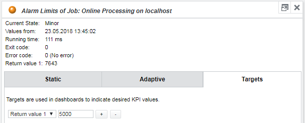
Click the + button and choose one of the available values from the dropdown. After that, the desired value can be set in the respective field, 5000 in the example above. The following value history widget shows the configured target as dotted line, starting from the time it was configured. Targets, like alarm limits, are time-dependent. This way, value histories can always be displayed with their alarm limits and targets they had in a certain point of time.