Forecasting

Overview

Identified language mismatch and prepared English refinement

SKOOR's forecasting module offers ML-based prediction of future trends on time series data. Four models are available:

• Prophet (See official documentation here)

• SARIMAX (See official documentation here)

• Linear Regression (See official documentation here)

• XGBoost (See official documentation here)

All models support datetime-indexed series sourced directly from a SKOOR DataSource or DataQuery. 

Forecasting Page

The forecasting page is divided into two sections. 

General Page

This section includes the settings of the forecasts.

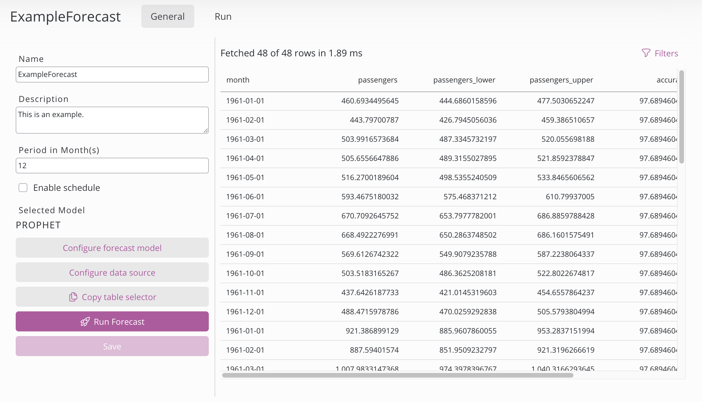
On the left side:

On the right side is the overview of the forecast data in a table. It’s only shown if already forecast exists.

Run Page

This section is responsible for running and monitor the runs of the forecast. It offers control over the history and enables insights.

Running a forecast can be done by clicking on the run forecast button. The complete history of runs can be deleted by clicking the delete jobs history button. Note that any tables created by the forecasts will be deleted and to get them again you have to run the forecast again. When a job is still running it can be cancelled by clicking on the red X on the right side of the shown status.

When clicking on a job, the console output, progress, status and further Information can be seen. In the console output, every group and its accuracy is printed out. The printed Accuracy is measured with WAPE (Weighted Absolute Percentage Error), is shown in percentages and is calculated on the performance of the model on the historical data.

Creating a forecast

A forecast configuration can be created by either clicking the Plus button on the left side and insert a name or by importing a forecast using the json-format. When a forecast configuration has been created, a few settings need to be set on the general page.

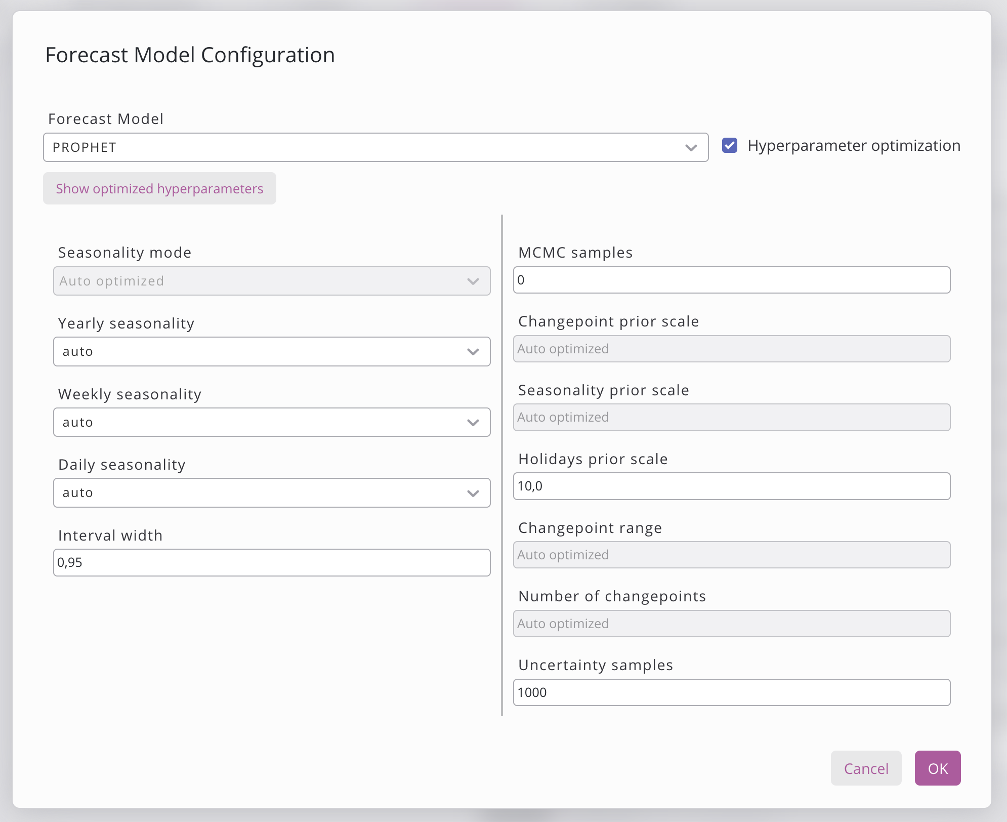
Model configuration

Clicking the 'Configure forecast model' button opens a dialogue box where the model can be chosen. Currently, there are 4 different model options that can be seen below. Some of the models feature a Hyperparameter optimisation button that allows the model to test various combinations of hyperparameters in order to find the best one. Various hyperparameters that can be set are listed below the model. If the hyperparameter search has already been triggered, you can view and copy the hyperparameters by clicking the 'Show optimized hyperparameters' button.

Once you have finished setting the hyperparameters, click Save to save the model configuration or Cancel to undo the changes.

Following models are available to choose from:

Prophet

• Prophet is a Machine Learning based open-source tool developed by Meta (former Facebook) for forecasting time series data. It’s designed to be robust to missing data and shifts in the trend, and particularly excels at forecasting time series with strong seasonality. Prophet can automatically handle holiday effects and allows the user to set own hyperparameters to make it even more precise.

• Prophet is the most widely used of the available options because it takes a moderate amount of time to train but it consistently delivers the best results, making it the most cost-effective choice in most scenarios. Prophet excels when given multiple seasons of data in which a recurrent seasonal effects, holiday effects or irregular trend shifts take place.

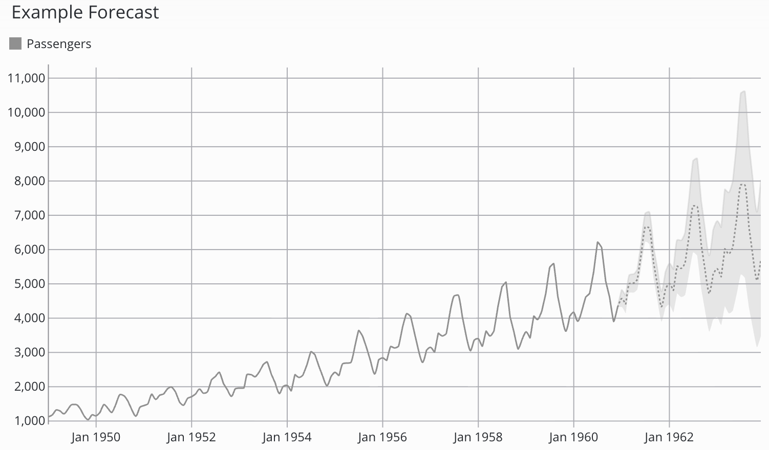
• When chosen, the prophet model also shows confidence interval bands, which indicates the certainty of the model in its predictions. When visualised on the dashboard, the confidence interval band is shown in a lighter color around the forecast.

  

The following variables can be configured:

SARIMAX

• SARIMAX (Seasonal Autoregressive Integrated Moving Average with Exogenous Regressors) is a statistical model used to predict future points based on past data. It handles both trends and seasonal patterns. It’s the extension of the ARIMA model by adding seasonal components.

• SARIMAX especially works when the data is generated stable and consistent and where a statistical model is preferred over a machine learning model.

There are no variables in the SARIMAX model that can be tuned by the User.

Linear Regression

• Linear Regression is used to predict trends only by fitting a straight line onto the training data and expanding this line into the future. It is a powerful tool to predict future trends in any time series data.

• Linear Regression is best used when the underlying data exhibits a clear, consistent linear trend with minimal seasonality or noise.

There are no variables in the Linear Regression model that can be tuned by the User.

XGBoost

• The XGBoost model uses gradient-boosted decision trees for direct multi-step forecasting. Before training, it applies extensive feature engineering to the input time series, extracting lag features, rolling statistics and calendar-based features, and then predicts each future point independently.

• XGBoost works best with complex, non-linear data. It can reach good accuracy but takes time to train and in some cases, the data has to be preprocessed separately beforehand.

The following variables can be configured:

Data Source

The configure data source window allows you to specify the data used to train the model.

The data source can be chosen on the left. There are two types of data source: a data source from your SKOOR database or a data query from the Data Query tab. Additional choices are required when selecting the data source and can be set in the window, such as the data source, table and columns. When selecting the data query option, the data query needs to be set, as well as the columns from that data query.

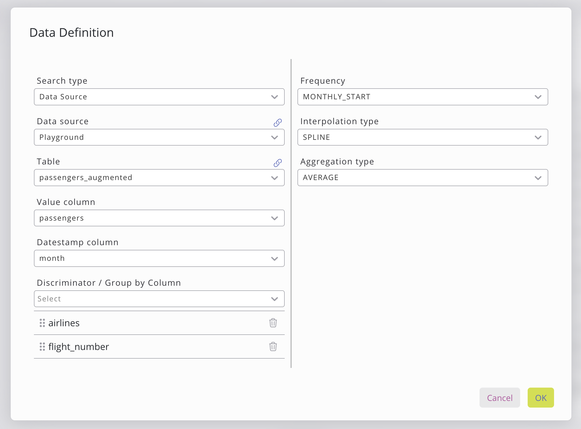
Value, date stamp and discriminator columns can be selected by clicking on the dropdown. The dropdown will automatically show columns that meet the requirements. Following columns needs to be chosen:

On the right side of the data window, further data preprocessing can be chosen.

Frequency

The frequency will set the output of the forecast. The following frequencies can be chosen:

Internally, the dataseries that is provided is being interpolated or aggregated to the set frequency using the interpolation type and/or aggregation type. Note that if your data has any missing date stamp in between or has too many for the frequency, the selected interpolation and/or aggregation is applied automatically to ensure a smooth forecasting.

Interpolation types:

Aggregation types:

Permissions

Readonly

• Read forecast results

• Search forecast configs by value definition

Editor

• Everything Readonly can do

• List all forecast configs (simple view only)

Dataeditor

• Everything Editor can do

• Full rights (create, read, update, delete) on forecast configs and groups

• Start, view, and cancel forecast jobs

• Export / import configs

Admin

• Everything Dataeditor can do

• Delete job history

Showing the Forecast on a Dashboard

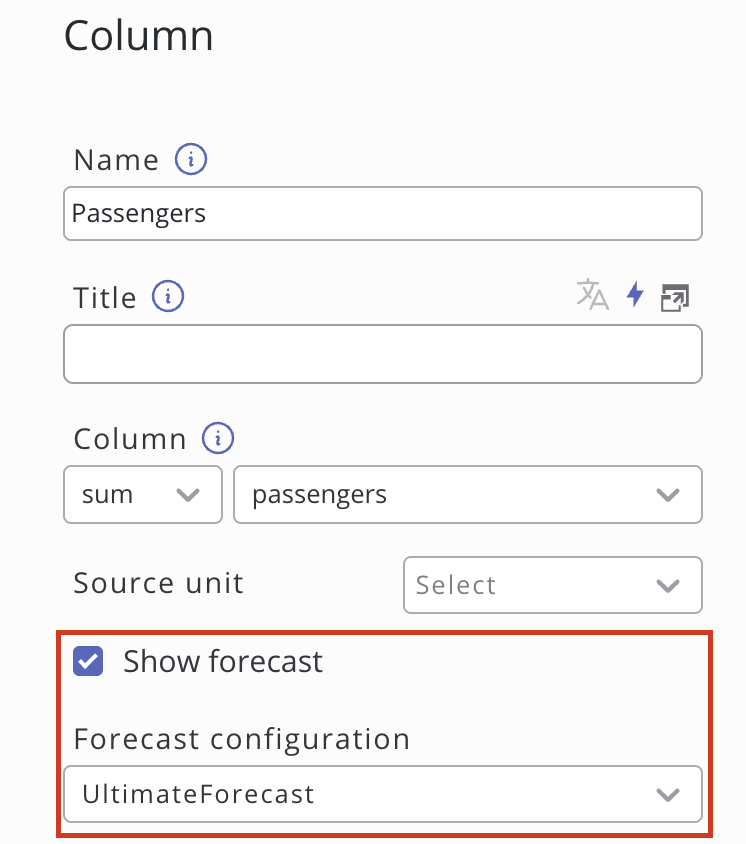
Using the default forecast widget

SKOOR implements an easy access to the forecast by introducing a button in the charts widget. Simply create a chart widget on the dashboard, set the chart type to Mixed and configure the same data definitions as in the forecast configuration. After setting up the datasource, either click on sync columns at the Columns sections on the bottom right in the widget edit dialogue or add the column that has been forecasted manually. Then click on that column and tick the show forecast box. Select the matching forecast configuration from the drop-down then apply. Now, the preview should already show the historical data with the matching forecast.

Using a custom Data Query

The table that contain the forecasting results can be copied to the clipboard by simply clicking on the copy table selector on the forecast configuration general page. Using this table, you can access the forecasting data and write your own data query e.g. in the SKOOR Studio. Note, that there are differences in the table columns as described:

• Prophet

  • value column (Named the same as the input value column.)

  • date stamp column (Named the same as the input datestamp column.)

  • lower confidence value (Named the same as the input value column but with “_lower” in the end.)

  • upper confidence value (Named the same as the input value column but with “_upper” in the end.)

  • accuracy

  • discriminator columns (Same number of columns as the number of discriminator columns given. Named the same as the input discriminator columns.)

• Linear Regression

  • value column (Named the same as the input value column.)

  • date stamp column (Named the same as the input datestamp column.)

  • accuracy

  • discriminator columns (Same number of columns as the number of discriminator columns given. Named the same as the input discriminator columns.)

• SARIMAX

  • value column (Named the same as the input value column.)

  • date stamp column (Named the same as the input datestamp column.)

  • accuracy

  • discriminator columns (Same number of columns as the number of discriminator columns given. Named the same as the input discriminator columns.)

• XGBoost

  • value column (Named the same as the input value column.)

  • date stamp column (Named the same as the input datestamp column.)

  • accuracy

  • discriminator columns (Same number of columns as the number of discriminator columns given. Named the same as the input discriminator columns.)